Plot Spectra

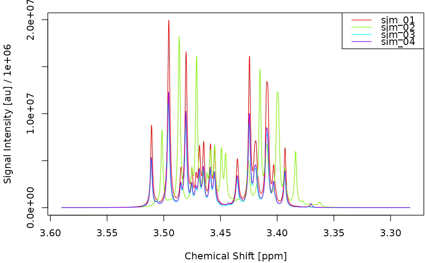
Plot a set of deconvoluted spectra.

Usage

plot_spectra(
  x,
  foc_rgn = NULL,
  what = NULL,
  sfy = 1e+06,
  cols = NULL,
  lty = NULL,
  names = NULL,
  xlab = "Chemical Shift [ppm]",
  ylab = paste("Signal Intensity [au] /", sfy),
  mar = c(4.1, 4.1, 1.1, 0.1),
  lgd = TRUE,
  main = NULL,
  xaxt = "s",
  yaxt = "s"
)

Arguments

x

An object of type decons0, decons1 or decons2. For details see metabodeconplus-classes.

foc_rgn

Numeric vector of length 2 specifying the focus region in ppm (e.g. c(3.55, 3.35)). If NULL (default), the full spectrum is shown.

what

Which signal to plot: "supal" (aligned superposition, default with fallback to "sup" then "si"), "sup" (superposition) or "si" (raw).

sfy

Scaling factor for the y-axis.

cols

Character vector of colors, one per spectrum. Defaults to rainbow(n).

lty

Line type(s), one per spectrum. Recycled if shorter than n. Defaults to 1 (solid) for all spectra.

names

Character vector of legend labels. Defaults to spectrum names.

xlab

Label for the x-axis.

ylab

Label for the y-axis.

mar

A numeric vector of length 4, which specifies the margins of the plot.

lgd

Logical or list. If TRUE, a legend is drawn at "topright" with cex = 0.8. If a list, its elements are passed to graphics::legend() to override position, size, etc. Pass lgd = FALSE to hide.

main

Optional plot title. Drawn via graphics::title().

xaxt, yaxt

Character. "s" (default) draws the axis normally; "n" suppresses axis ticks and tick labels. Passed to graphics::plot().

Value

A plot of the deconvoluted spectra.

See also

plot_spectrum() for a much more sophisticated plotting routine suitable for plotting a single spectrum.

Author

2024-2025 Tobias Schmidt: initial version.

Examples

x <- deconvolute(sim[1:4], sfr = c(3.55, 3.35))
#> 2026-08-09 09:53:20.45 Starting deconvolution (spectra: 4, workers: 1)
#> 2026-08-09 09:53:20.45 Starting deconvolution of sim_01 using R backend
#> 2026-08-09 09:53:20.45 Starting peak selection
#> 2026-08-09 09:53:20.45 Detected 312 peaks
#> 2026-08-09 09:53:20.45 Removing peaks with low scores
#> 2026-08-09 09:53:20.46 Removed 285 peaks
#> 2026-08-09 09:53:20.46 Fitting Lorentz curves (3 iterations)
#> 2026-08-09 09:53:20.46 Finished deconvolution of sim_01
#> 2026-08-09 09:53:20.46 Starting deconvolution of sim_02 using R backend
#> 2026-08-09 09:53:20.46 Starting peak selection
#> 2026-08-09 09:53:20.46 Detected 316 peaks
#> 2026-08-09 09:53:20.46 Removing peaks with low scores
#> 2026-08-09 09:53:20.46 Removed 286 peaks
#> 2026-08-09 09:53:20.46 Fitting Lorentz curves (3 iterations)
#> 2026-08-09 09:53:20.46 Finished deconvolution of sim_02
#> 2026-08-09 09:53:20.46 Starting deconvolution of sim_03 using R backend
#> 2026-08-09 09:53:20.46 Starting peak selection
#> 2026-08-09 09:53:20.46 Detected 333 peaks
#> 2026-08-09 09:53:20.46 Removing peaks with low scores
#> 2026-08-09 09:53:20.46 Removed 308 peaks
#> 2026-08-09 09:53:20.46 Fitting Lorentz curves (3 iterations)
#> 2026-08-09 09:53:20.46 Finished deconvolution of sim_03
#> 2026-08-09 09:53:20.46 Starting deconvolution of sim_04 using R backend
#> 2026-08-09 09:53:20.46 Starting peak selection
#> 2026-08-09 09:53:20.46 Detected 324 peaks
#> 2026-08-09 09:53:20.46 Removing peaks with low scores
#> 2026-08-09 09:53:20.47 Removed 298 peaks
#> 2026-08-09 09:53:20.47 Fitting Lorentz curves (3 iterations)
#> 2026-08-09 09:53:20.47 Finished deconvolution of sim_04
#> 2026-08-09 09:53:20.47 Finished deconvolution 0.014 secs
plot_spectra(x)