Get Started

This article shows how Metabodecon can be used for deconvoluting and aligning one-dimensional NMR spectra using the pre-installed Sim dataset as an example. The Sim dataset includes 16 simulated spectra, each with 2048 data points ranging from ≈ 3.6 to 3.3 ppm. These simulated spectra closely mimic the resolution and signal strength of real NMR experiments on blood plasma from 16 individuals. The Sim dataset is used instead of the Blood dataset because it is smaller, faster to process, and comes pre-installed with the package. For more information on the Sim and Blood datasets, see Datasets.

For an overview of the S3 classes used to represent spectra throughout the package (spectrum, decon2, align, and their collections), see ?metabodeconplus-classes.

Read spectra

Spectra are read from disk with read_spectrum() (single spectrum) or read_spectra() (a whole directory of spectra). Both support the Bruker and JCAMP-DX formats.

File structure

read_spectra() expects one of the two directory layouts shown below. For Bruker data, point data_path at the folder that contains the individual sample folders; each sample folder holds an experiment number (expno, e.g. 10) and, under pdata/, a processing number (procno, e.g. 10). For JCAMP-DX data, point data_path at the folder containing the .dx files.

C:/bruker/urine              # data_path (user input)
├── urine_1/                 # sample name (user input)
│   └── 10/                  # expno (called spectroscopy_value here)
│       ├── acqus            # acquisition parameters (constant)
│       └── pdata/
│           └── 10/          # procno (called processing_value here)
│               ├── 1r       # real part of the processed spectrum (constant)
│               └── procs    # processing parameters (constant)
├── urine_2/...
└── ...
C:/jcampdx/urine             # data_path (user input)
├── urine_1.dx               # one .dx file per sample (user input)
├── urine_2.dx
└── ...

Deconvolute spectra

To find the path to the Sim dataset, you can use the metabodeconplus_file() function, which returns the path to any file or directory within the package directory. To deconvolute the spectra within the Sim dataset you can read them into R using read_spectra() and then call deconvolute() as follows:

sim_dir <- metabodeconplus::metabodeconplus_file("bruker/sim")
sim <- metabodeconplus::read_spectra(sim_dir)
deconvoluted_spectra <- metabodeconplus::deconvolute(
    sim,                 # The object containing spectra
    sfr = c(3.35, 3.55), # Borders of signal free region (SFR) in ppm
    smit = 2, smws = 5,  # Smoothing parameters
    verbose = FALSE      # Disable verbose output
)

The provided parameters are used directly for the deconvolution of all spectra. To verify that the signal-free region was set correctly and to assess the quality of the deconvolution, use plot_spectrum() after the call (see below).

Visualize deconvoluted spectra

After completing the deconvolution, it is advisable to visualize the extracted signals using plot_spectrum() to assess the quality of the deconvolution.

# Visualize the first spectrum.
metabodeconplus::plot_spectrum(deconvoluted_spectra[[1]])

# Visualize the second spectrum, this time without the legend.
metabodeconplus::plot_spectrum(deconvoluted_spectra[[1]], lgd = FALSE)

# Visualize all spectra and save them to a pdf file
pdfpath <- tempfile(fileext = ".pdf")
pdf(pdfpath)
for (x in deconvoluted_spectra) {
    metabodeconplus::plot_spectrum(x, main = x$filename)
}
dev.off()
cat("Plots saved to", pdfpath, "\n")

Out of the 16 generated plots, the first two are shown as examples in Figure 2. Things to look out for are:

1. That the smoothing does not remove any real signals. If the smoothing is too strong, i.e., the smoothed signal intensity (SI) is very different from the raw SI, you should adjust the smoothing parameters smit and smws in the call to deconvolute().
2. That the superposition of the lorentz curves is a good approximation of the smoothed SI. If major peaks are missed by the algorithm, you should reduce the threshold delta in the call to deconvolute().

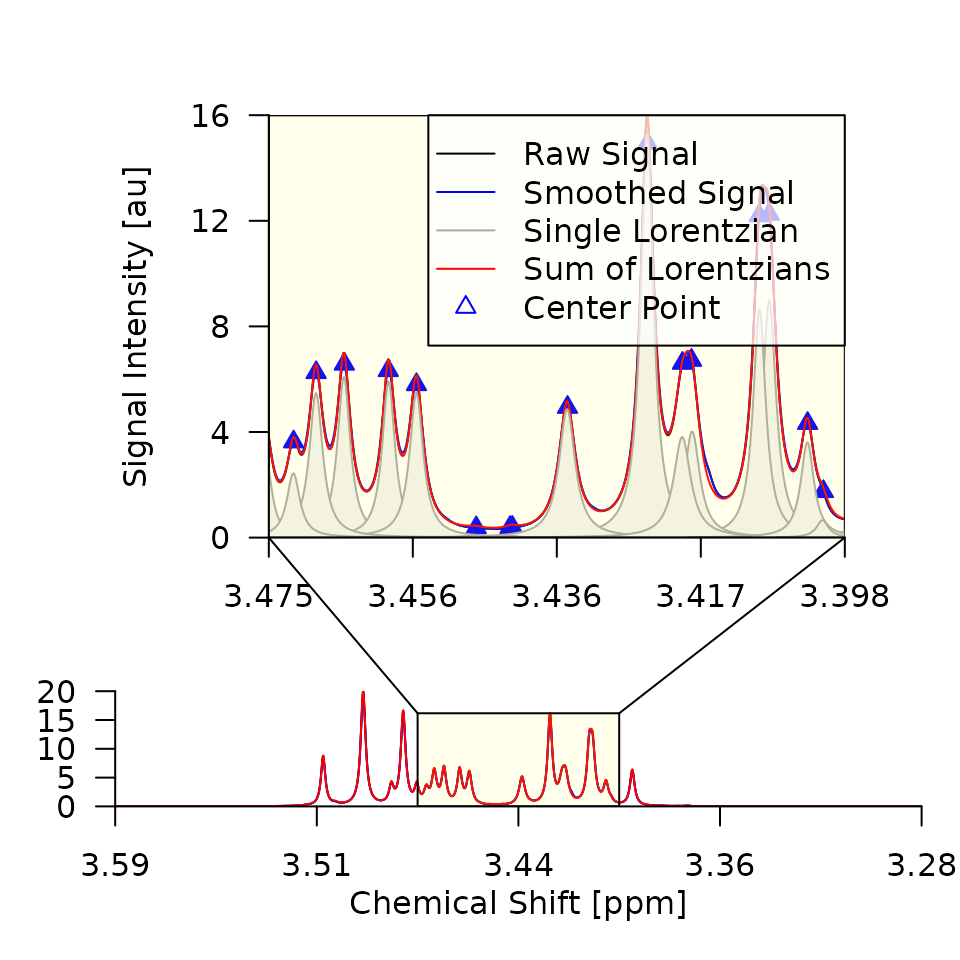
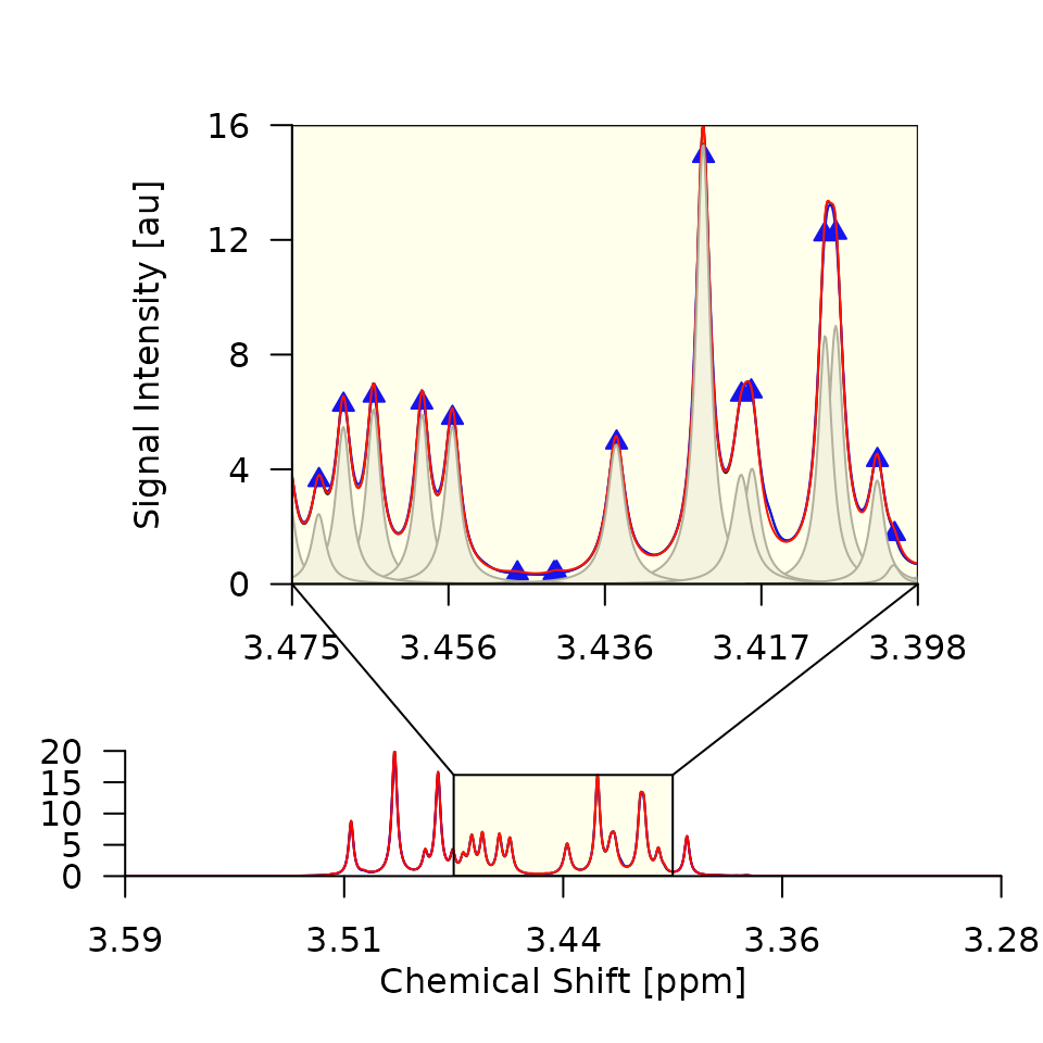
Figure 2. Deconvolution results for the first two spectra of the Sim dataset. The raw SI (black), smoothed SI (blue), and superposition of Lorentz curves (red) are closely aligned, indicating that smit/smws and delta were chosen well and that the deconvolution was successful.

Align deconvoluted spectra

The last step in the Metabodecon Workflow is to align the deconvoluted spectra. This is necessary because the chemical shifts of the peaks in the spectra may vary slightly due to differences in the measurement conditions.

To perform the alignment, you can use align(). To visualize the data before and after the alignment, you can use plot_spectra():

# Plot spectra before alignment. Only show spectra 1-8 for clarity.
metabodeconplus::plot_spectra(deconvoluted_spectra[1:8], lgd = FALSE)

# Align spectra and plot again.
aligned_spectra <- metabodeconplus::align(deconvoluted_spectra)
metabodeconplus::plot_spectra(aligned_spectra[1:8])

The resulting plots are shown in Figure 3. Before the alignment, the spectra exhibit generally similar shapes but do not perfectly overlap. After the alignment, the spectra are much more consistent with each other, indicating that the alignment was successful. Notably, spectrum two has been shifted significantly to the left.

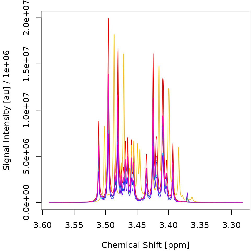
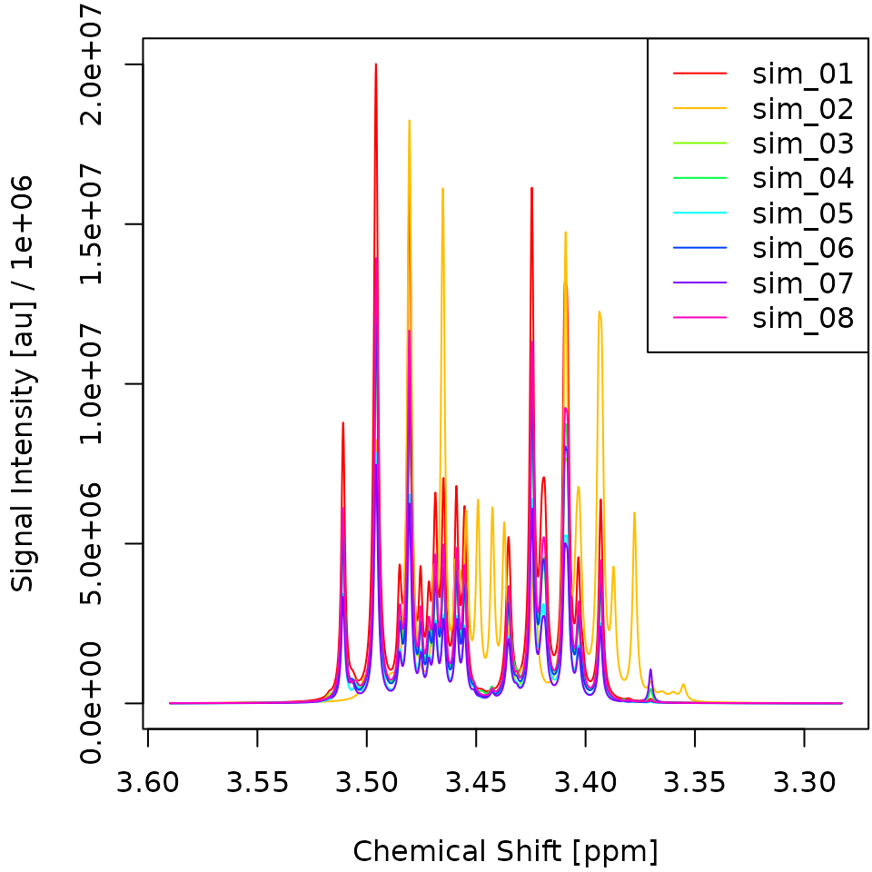
Figure 3. Overlay of the first eight deconvoluted spectra from the Sim dataset before alignment (left) and after alignment (right). The x-Axis gives the chemical shift of each datapoint in parts per million (ppm). The y-Axis gives the signal intensity of each datapoint in arbitrary units (au). All specta are pretty similar to each other except for Spectrum 2, which got shifted approx. 0.01 ppm to the right.