GUI Usage

This tutorial shows how to start the FastRet GUI and use its four modes.

Starting the GUI

Install the package and run this in an interactive R session:

FastRet::start_gui()

The console prints:

Listening on http://localhost:8080

Open http://localhost:8080 in your browser to use the GUI.

The GUI has four modes, shown as tabs at the top: Train, Select, Adjust and Predict. Hover over a tab to see its full name. Click the question-mark icon next to any input for a short help text.

If start_gui() reports a CDK version error, FastRet needs CDK 2.9 or newer and a working Java installation. See the Installation article for how to set up Java and rcdk.

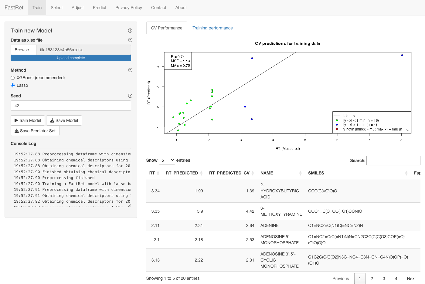
Train new Model

Use the Train tab to build a model from your own measurements: an Excel file with the names, SMILES and retention times of metabolites measured on your column. FastRet ships an example file with 442 metabolites measured on a reverse-phase column (35 °C, 0.3 ml/min). To see its path and contents:

path <- system.file("extdata", "RP.xlsx", package = "FastRet")
cat(path, "\n", sep = "")
#> /home/runner/work/_temp/Library/FastRet/extdata/RP.xlsx
df <- openxlsx::read.xlsx(path, 1)
head(df)
#>     RT                                                    SMILES
#> 1 3.34                                              CCC(C(=O)O)O
#> 2 3.35                                     COC1=C(C=CC(=C1)CCN)O
#> 3 2.11                                    C1=NC2=C(N1)C(=NC=N2)N
#> 4 2.10          C1=NC2=C(C(=N1)N)N=CN2C3C(C(C(O3)COP(=O)(O)O)O)O
#> 5 3.13             C1C2C(C(C(O2)N3C=NC4=C3N=CN=C4N)O)OP(=O)(O1)O
#> 6 2.07 C1=NC2=C(C(=N1)N)N=CN2C3C(C(C(O3)COP(=O)(O)O)OP(=O)(O)O)O
#>                                   NAME
#> 1                2-HYDROXYBUTYRIC ACID
#> 2                    3-METHOXYTYRAMINE
#> 3                              ADENINE
#> 4           ADENOSINE 5'-MONOPHOSPHATE
#> 5 ADENOSINE 3',5'-CYCLIC MONOPHOSPHATE
#> 6          ADENOSINE 3',5'-DIPHOSPHATE

Set the controls, then click Train Model:

1. Data as xlsx file — your Excel file (columns RT, NAME, SMILES).
2. Method — XGBoost (recommended) or Lasso.
3. Seed — random seed. Keep the default (42) for reproducible results.

The Console Log shows progress. When training finishes, the main panel shows the cross-validation and training plots and a table of predictions. For the details, see Model-Training in the Package-Internals article.

Two buttons then appear: Save Model (an .rds file) and Save Predictor Set (the training data with descriptors). To predict with your model, save it, switch to the Predict tab, upload it there, enter your SMILES and click Predict (see Predict Retention Times).

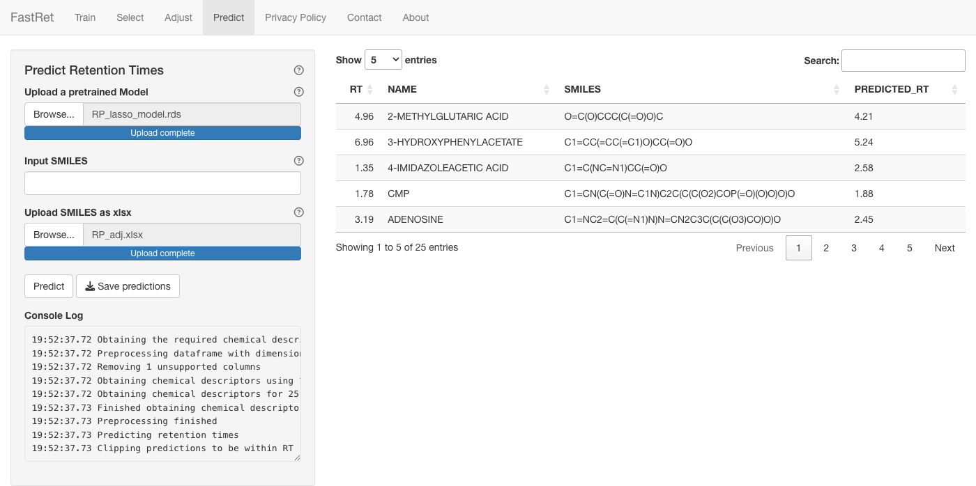
Predict Retention Times

Use a saved model to predict retention times for new molecules:

1. Upload the model under Upload a pretrained Model.
2. Enter a SMILES in Input SMILES, or upload an Excel file (columns NAME, SMILES) under Upload SMILES as xlsx.
3. Click Predict.

The predictions appear as a table in the main panel. Click Save predictions to download them as an Excel file.

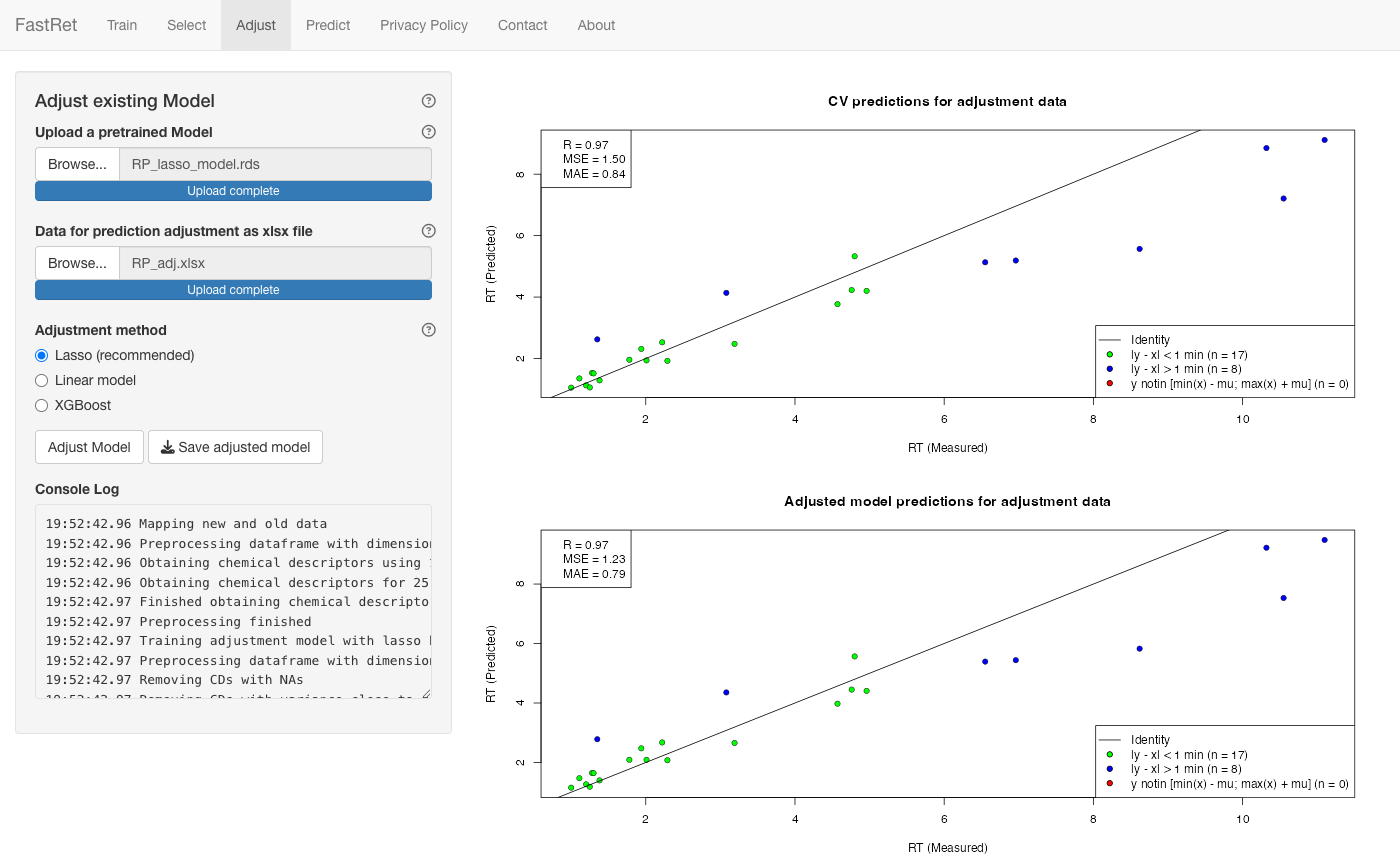
Adjusting existing model

If you re-measured some metabolites on a new column that were also measured on the original one, use the Adjust tab to adapt an existing model to the new column:

1. Upload the model under Upload a pretrained Model.
2. Upload the re-measured metabolites (columns RT, NAME, SMILES) under Data for prediction adjustment as xlsx file.
3. Choose the Adjustment method: Lasso (recommended), Linear model or XGBoost. Lasso and XGBoost use the base retention time and the molecular descriptors, so they can capture compound-specific shifts; the linear model fits a straight-line correction from the base retention time alone.
4. Click Adjust Model.

The main panel shows the performance of the adjusted model. Click Save adjusted model to download it. Use it like any other model on the Predict tab.

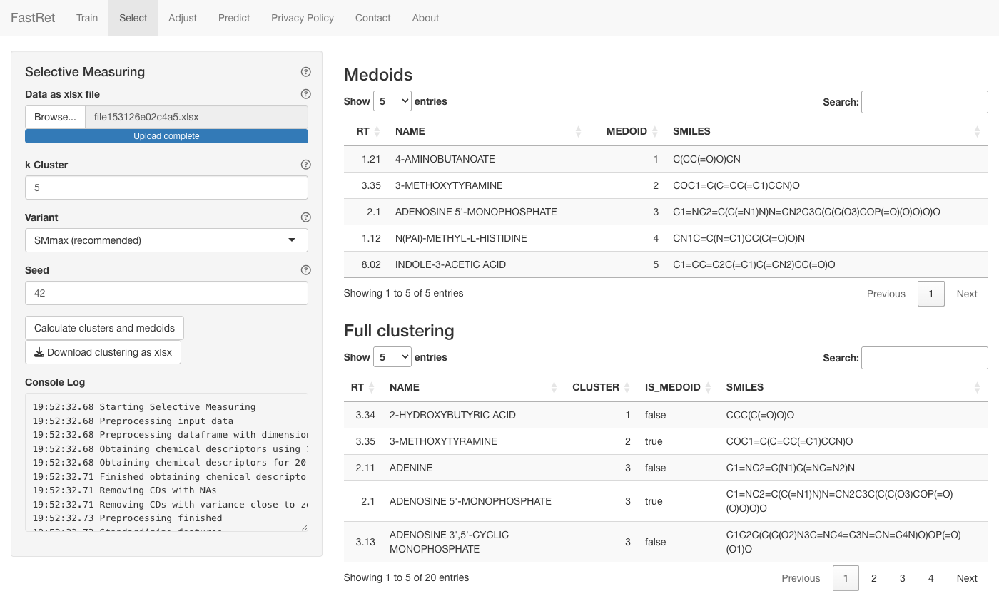
Selective Measuring

Adjusting a model to a new column needs a few metabolites measured on that column. The Select tab picks the k most representative molecules to measure, so you cover the diversity of your dataset with as little lab work as possible. It uses Ridge Regression and PAM (k-medoids) clustering.

1. Upload an Excel file (columns NAME, SMILES, RT).
2. k Cluster — how many molecules to select.
3. Variant — how strongly the retention time guides the selection: SMmax (default, weighted like the most important descriptor), SM1 (unscaled), SM0 (excluded) or SMinf (retention time only). The info button explains each.
4. Seed — random seed. Keep the default (42) for a reproducible selection.
5. Click Calculate clusters and medoids.
6. Click Download clustering as xlsx to save the selected molecules and their clusters.

The main panel lists the selected molecules and the full clustering. Measure the selected molecules on the new column, then use them to adjust your model.