Draws a single spectrum. Internally used by plot_spectrum(), which is
usually the recommended way to plot spectra. For usage examples see
test/testthat/test-draw_spectrum.R.
![[Experimental]](figures/lifecycle-experimental.svg)
Usage
draw_spectrum(
  obj,
  foc_rgn = NULL,
  foc_frac = NULL,
  foc_only = TRUE,
  add = FALSE,
  fig_rgn = NULL,
  main = NULL,
  show = TRUE,
  show_d2 = FALSE,
  truepar = NULL,
  mar = c(4.1, 5.1, 1.1, 1.1),
  sf_vert = "auto",
  si_line = list(),
  sm_line = list(),
  sp_line = list(),
  d2_line = list(),
  al_line = list(),
  lc_lines = list(),
  tp_lines = list(),
  al_lines = list(),
  cent_pts = list(),
  bord_pts = list(),
  norm_pts = list(),
  tp_pts = list(),
  fp_pts = list(),
  miss_pts = list(),
  bg_rect = list(),
  foc_rect = list(),
  lc_rects = list(),
  tp_rects = list(),
  bt_axis = list(),
  lt_axis = list(),
  tp_axis = list(),
  rt_axis = list(),
  bt_text = list(),
  lt_text = list(),
  tp_text = list(),
  rt_text = list(),
  tp_verts = list(),
  lc_verts = list(),
  al_verts = list(),
  ze_hline = list(),
  al_arrows = list(),
  lgd = list()
)
Arguments
- obj
An object of type
spectrumordecon2. For details see Metabodecon Classes.- foc_rgn
Numeric vector specifying the start and end of focus region in ppm.
- foc_frac
Numeric vector specifying the start and end of focus region as fraction of the full spectrum width.
- foc_only
Logical. If TRUE, only the focused region is drawn. If FALSE, the full spectrum is drawn.
- add
If TRUE, draw into the currently open figure. If FALSE, start a new figure.
- fig_rgn
Drawing region in normalized device coordinates as vector of the form
c(x1, x2, y1, y2).- main
Main title of the plot. Drawn via
title().- show
Logical. If FALSE, the function returns without doing anything.
- show_d2
Logical. If TRUE, the second derivative of the spectrum is drawn. Setting this to TRUE changes most of the defaults for the drawing, e.g. by disabling the drawing of anything related to signal intensities and by changing the y-axis label to "Second Derivative".
- truepar
Data frame with columns x0, A and lambda containing the true lorentzian that were used to simulate the spectrum. Required if any
tp_*argument is set.- mar
Number of lines below/left-of/above/right-of plot region.
- sf_vert
Scale factor for vertical lines corresponding to
lc_verts,tp_vertsandal_verts. If a numeric value is provided, the height of each line equals the area of the corresponding lorentzian curve multiplied bysf_vert. In addition, the following strings are supported:"auto": A suitable numeric value forsf_vertis chosen automatically, in a way that the highest integral equals the highest signal intensity after multiplication withsf_vert."peak": Vertical lines are drawn from bottom to top of the corresponding peak."full": Vertical lines are drawn over the full vertical range of the plot region.
- si_line, sm_line, sp_line, al_line, d2_line, lc_lines, tp_lines, al_lines
List of parameters passed to
lines()when drawing the raw signal intensities (si_line), smoothed signal intensities (sm_line), superposition of lorentzian curves (sp_line), aligned lorentzian curves (al_line), second derivative (d2_line), lorentzian curves found by deconvolution (lc_lines), true lorentzian curves (tp_lines) and aligned lorentzian curves (al_lines), respectively.- cent_pts, tp_pts, fp_pts, miss_pts, bord_pts, norm_pts
List of parameters passed to
points()when drawing the peak center points, true positive peaks, false positive peaks, missed peaks, peak border points and non-peak points.- bg_rect, lc_rects, foc_rect, tp_rects
List of parameters passed to
rect()when drawing the background, lorentzian curve substitutes, focus rectangle and/or true lorentzian curve substitutes.- bt_axis, lt_axis, tp_axis, rt_axis
List of parameters used to overwrite the default values passed to
axis()when drawing the bottom, left, top and right axis. In addition to the parameters ofaxis(), the following additional parameters are supported as well:n: Number of tickmarks.digits: Number of digits for rounding the labels. If a vector of numbers is provided, all numbers are tried, untilnunique labels are found. See 'Details'.sf: Scaling factor. Axis values are divided by this number before the labels are calculated. If you set this to anything unequal 1, you should also set the corresponding margin text in a way that reflects the scaling. Example: by default, a scaling factor of 1e6 is used for drawing signal intensities and a scaling factor of 1 for drawing the second derivative. To make clear, that the user should be careful when interpreting the signal intensity values, the corresponding margin text is set to "Signal Intensity [au]" where "au" means "Arbitrary Units", indicating that the values might be scaled.
- bt_text, lt_text, tp_text, rt_text
List of parameters used to overwrite the default values passed to
mtext()when drawing the bottom, left, top and right margin texts (i.e. the axis labels).- lc_verts, tp_verts, al_verts
List of parameters passed to
segments()when drawing vertical lines at the centers of estimated, true or aligned lorentzian curves. Settingtp_verts$showto TRUE requirestrueparto be set.- ze_hline
List of parameters passed to
abline()when drawing a horizontal line at y = 0.- al_arrows
List of parameters passed to
arrows()when drawing arrows between the estimated and aligned lorentzian curve centers.- lgd
List of parameters passed to
legend()when drawing the legend.
Details
Parameters bt_axis, lt_axis, tp_axis and rt_axis all support option
n and digits, where n = 5 means "Draw 5 tickmarks over the full axis
range" and digits = 3 means "round the label shown beside each tickmark to
3 digits". If n or digits is omitted, a suitable value is chosen
automatically. Providing a vector of digits causes each digit to be tried
until a digit is encountered that results in n unique labels. Example:
Assume we have n = 4 and the corresponding calculated tickmark positions
are: 1.02421, 1.02542, 1.02663 and 1.02784. If we provide digits = 1:5, the
following representations are tried:
| digit | label 1 | label 2 | label 3 | label 4 |
| 1 | 1.0 | 1.0 | 1.0 | 1.0 |
| 2 | 1.02 | 1.03 | 1.03 | 1.03 |
| 3 | 1.024 | 1.025 | 1.027 | 1.028 |
| 4 | 1.0242 | 1.0254 | 1.0266 | 1.0278 |
| 5 | 1.02421 | 1.02542 | 1.02663 | 1.02784 |
In the above example the process would stop at digit = 3, because at this
point we have n = 4 unique labels (1.024, 1.025, 1.027 and 1.028).
Examples
decon <- deconvolute(sim[[1]], sfr = c(3.55, 3.35))
#> 2026-07-20 06:55:42.14 Starting deconvolution of 1 spectrum using 1 worker
#> 2026-07-20 06:55:42.14 Starting deconvolution of sim_01 using R (legacy) backend
#> 2026-07-20 06:55:42.14 Removing water signal
#> 2026-07-20 06:55:42.14 Removing negative signals
#> 2026-07-20 06:55:42.14 Smoothing signals
#> 2026-07-20 06:55:42.15 Starting peak selection
#> 2026-07-20 06:55:42.15 Detected 314 peaks
#> 2026-07-20 06:55:42.15 Removing peaks with low scores
#> 2026-07-20 06:55:42.15 Removed 287 peaks
#> 2026-07-20 06:55:42.15 Initializing Lorentz curves
#> 2026-07-20 06:55:42.15 MSE at peak tiplet positions: 4.0838805770844048836921
#> 2026-07-20 06:55:42.15 Refining Lorentz Curves
#> 2026-07-20 06:55:42.16 MSE at peak tiplet positions: 0.1609359876216345797140
#> 2026-07-20 06:55:42.16 MSE at peak tiplet positions: 0.0228015051613790278862
#> 2026-07-20 06:55:42.16 MSE at peak tiplet positions: 0.0071638016610617982066
#> 2026-07-20 06:55:42.16 Formatting return object as decon2
#> 2026-07-20 06:55:42.16 Finished deconvolution of sim_01
#> 2026-07-20 06:55:42.16 Finished deconvolution of 1 spectrum in 0.019 secs
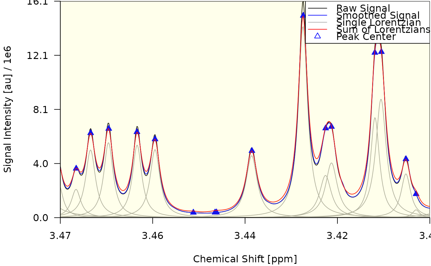
draw_spectrum(obj = decon)
 #> $plt_rgn_ndc
#> [1] 0.153 0.967 0.123 0.967
#>
#> $foc_rgn_ndc
#> [1] 0.9675974 0.1524026 0.1230000 0.9670000
#>
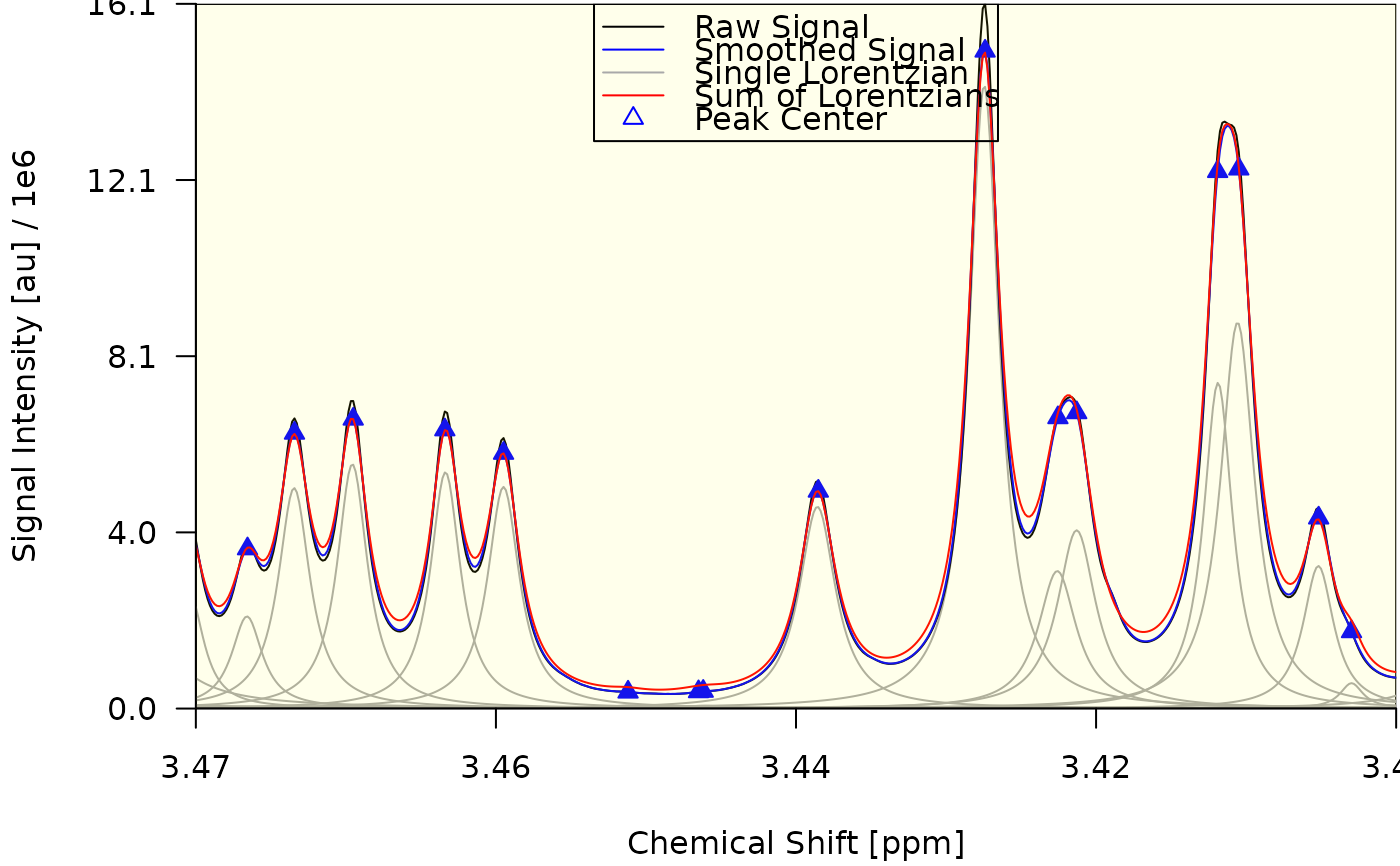
draw_spectrum(obj = decon, lgd = list(x = "top", bg = NA))
#> $plt_rgn_ndc
#> [1] 0.153 0.967 0.123 0.967
#>
#> $foc_rgn_ndc
#> [1] 0.9675974 0.1524026 0.1230000 0.9670000
#>
draw_spectrum(obj = decon, lgd = list(x = "top", bg = NA))
 #> $plt_rgn_ndc
#> [1] 0.153 0.967 0.123 0.967
#>
#> $foc_rgn_ndc
#> [1] 0.9675974 0.1524026 0.1230000 0.9670000
#>
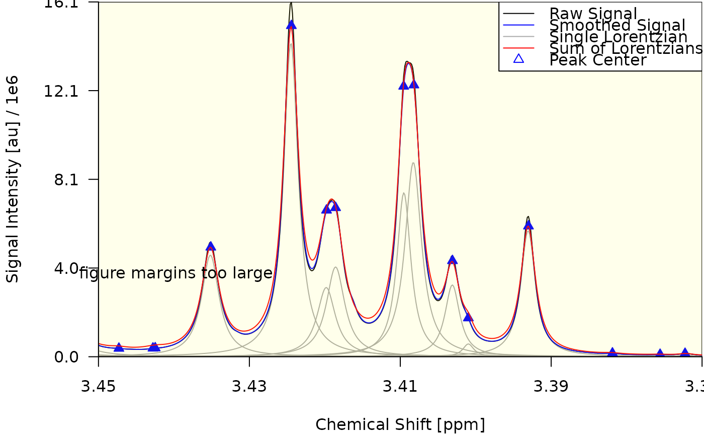
draw_spectrum(obj = decon, foc_rgn = c(3.45, 3.37))
#> $plt_rgn_ndc
#> [1] 0.153 0.967 0.123 0.967
#>
#> $foc_rgn_ndc
#> [1] 0.9675974 0.1524026 0.1230000 0.9670000
#>
draw_spectrum(obj = decon, foc_rgn = c(3.45, 3.37))
 #> $plt_rgn_ndc
#> [1] 0.153 0.967 0.123 0.967
#>
#> $foc_rgn_ndc
#> [1] 0.1519799 0.9680201 0.1230000 0.9670000
#>
draw_spectrum(obj = decon, add = FALSE, lgd = FALSE,
fig = c(.2, .8, .2, .4), mar = c( 0, 0, 0, 0))
#> $plt_rgn_ndc
#> [1] 0.2 0.8 0.2 0.4
#>
#> $foc_rgn_ndc
#> [1] 0.8004403 0.1995597 0.2000000 0.4000000
#>
draw_spectrum(obj = decon, add = TRUE, lgd = FALSE,
fig = c(0.2, 0.8, 0.6, 0.8), mar = c(0, 0, 0, 0))
#> $plt_rgn_ndc
#> [1] 0.153 0.967 0.123 0.967
#>
#> $foc_rgn_ndc
#> [1] 0.1519799 0.9680201 0.1230000 0.9670000
#>
draw_spectrum(obj = decon, add = FALSE, lgd = FALSE,
fig = c(.2, .8, .2, .4), mar = c( 0, 0, 0, 0))
#> $plt_rgn_ndc
#> [1] 0.2 0.8 0.2 0.4
#>
#> $foc_rgn_ndc
#> [1] 0.8004403 0.1995597 0.2000000 0.4000000
#>
draw_spectrum(obj = decon, add = TRUE, lgd = FALSE,
fig = c(0.2, 0.8, 0.6, 0.8), mar = c(0, 0, 0, 0))
 #> $plt_rgn_ndc
#> [1] 0.2 0.8 0.6 0.8
#>
#> $foc_rgn_ndc
#> [1] 0.8004403 0.1995597 0.6000000 0.8000000
#>
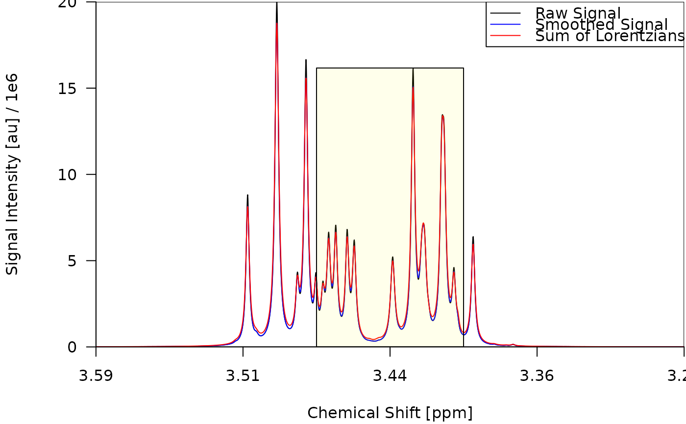
draw_spectrum(obj = decon, lc_lines = NULL, lc_rects = NULL, foc_only = FALSE)
#> $plt_rgn_ndc
#> [1] 0.2 0.8 0.6 0.8
#>
#> $foc_rgn_ndc
#> [1] 0.8004403 0.1995597 0.6000000 0.8000000
#>
draw_spectrum(obj = decon, lc_lines = NULL, lc_rects = NULL, foc_only = FALSE)
 #> $plt_rgn_ndc
#> [1] 0.153 0.967 0.123 0.967
#>
#> $foc_rgn_ndc
#> [1] 0.6617500 0.4582500 0.1230000 0.8052662
#>
#> $plt_rgn_ndc
#> [1] 0.153 0.967 0.123 0.967
#>
#> $foc_rgn_ndc
#> [1] 0.6617500 0.4582500 0.1230000 0.8052662
#>