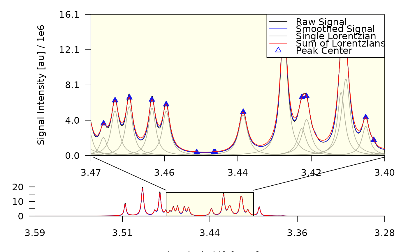
Arguments
- x
An object of type
spectrum,decon0,decon1,decon2oralign. For details see Metabodecon Classes.- ...
Additional arguments passed to
draw_spectrum()for every sub figure. See 'Details'.- obj
An object of type
spectrumordecon2. Usually auto generated fromx, but can be set manually in case the default conversion is not sufficient.- foc_frac
A numeric vector specifying the start and end of the focus region as fraction of the full spectrum width. Only used if
foc_rgnis set to NULL.- foc_rgn
A numeric vector specifying the start and end of the focus region in ppm. If set to NULL,
foc_fracis used to determine the focus region. If bothfoc_rgnand are set to NULL, a suitable focus region is chosen automatically. Takes precedence overfoc_frac.- sub1, sub2, sub3
List of arguments passed to
draw_spectrum()when drawing sub figure 1-3. See 'Details'.- mar
A numeric vector of length 4 specifying the margins of the plot. Passed to
par(). If set toNULL, a suitable value is chosen automatically.- frame
A list of values passed to
box()when drawing the frame around plot region. If set toNULL, no frame is drawn.- con_lines
A list of values passed to
lines()when drawing the connecting lines between sub figure 1 and the focus rectangle in sub figure 3. See 'Details'. If set toNULL, the connecting lines are not drawn.
Details
This function first initializes a new plotting canvas. After that it calls
draw_spectrum() multiple times to draw the following sub figures onto the
plotting canvas:
The signal intensities in the focus region
The second derivative in the focus region
The signal intensities over all datapoints
The argument lists for the individual calls to draw_spectrum() are
determined at runtime and depend on the arguments passed to plot_spectrum()
as well as the currently active graphics device. To customize the appearance
of the individual sub plots, you can overwrite each value passed to
draw_spectrum() by providing a corresponding named element in sub1,
sub2 or sub3.
A sketch of the resulting figure is shown below.
 __________________________________________
|        ______________1_____________      |
|       | Sub1: Signal Intensity in  |     |
|       | Focus Region               |     |
|       |             /\             |     |
|       |            /  \            |     |
|       |           /    \  /\       |     |
|     11|          /      \/  \      |7    |
|       |     /\  /            \     |     |
|       |    /  \/              \    |     |
|       |   /                    \   |     |
|       |__/___________0__________\__|     |
|       | Sub2: Second Derivative    |     |
|     11| in Focus Region            |7    |
|       |____________________________|     |
|                      3                   |
|    __________________3_________________  |
|   |  Sub3: Signal Intensity over all   | |
|   |  Datapoints     ________________   | |
| 5 |                | Focus Rectangle|  |1|
|   |     /\         |       /\       |  | |
|   |    /  \        |      /  \/\    |  | |
|   |   /    \   /\  |   /\/      \   |  | |
|   |__/______\_/__\_|__/__________\__|__| |
|______________________5___________________|
Note that the figure created by plot_spectrum() can be part of a
multi-figure configuration as created when setting mfrow or mfcol via
par(). Example:
_______________________________________
| Plot Spectrum with   | Other Figure  |
| sub3 = TRUE          | Other Figure  |
|      ___________     |  ___________  |
|     | Sub Fig 1 |    | | x      x  | |
|     |___________|    | |      x    | |
|     |_Sub_Fig_2_|    | |      x    | |
|   _________________  | |   x     x | |
|  |    Sub Fig 3    | | |      x    | |
|  |_________________| | |___________| |
|______________________|_______________|
| Some other Figure    | Plot Spectrum |
|                      | sub3 = FALSE  |
|  _________________   |  ___________  |
| |     ___         |  | | Sub Fig 1 | |
| | ___/   \___     |  | |           | |
| |/           \____|  | |___________| |
| |                 |  | | Sub Fig 2 | |
| |_________________|  | |___________| |
|______________________|_______________|Examples
## 1. Prepare a deconvoluted spectrum as input
spec <- read_spectrum(metabodecon_file("sim/sim_01"))
decon <- generate_lorentz_curves_sim(spec)
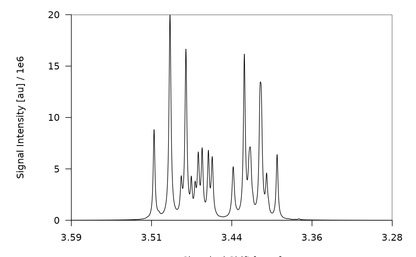
## 2.1. Plot the full (non-deconvoluted) spectrum
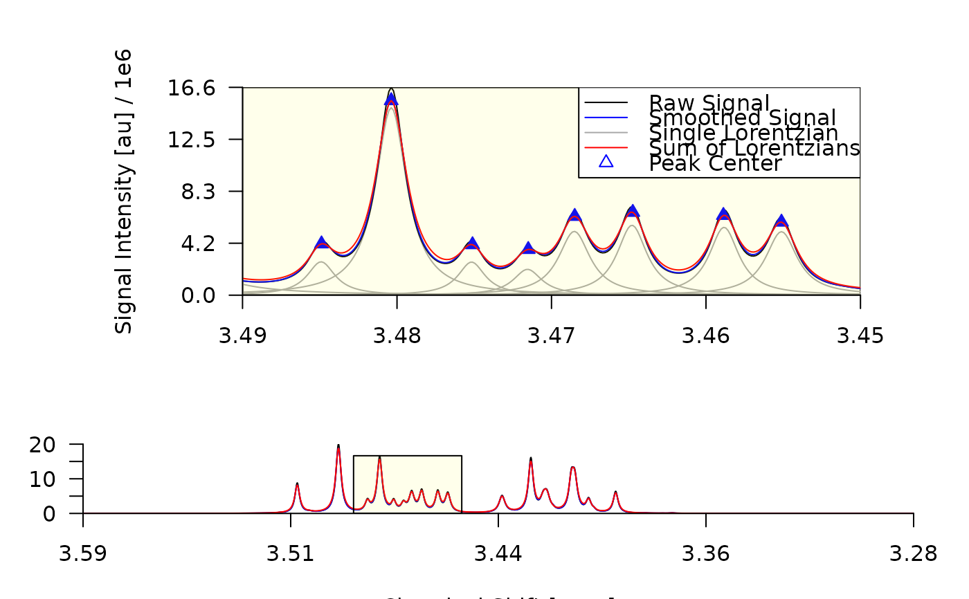
## 2.2. Remove connecting lines, and focus on a specific region specified in ppm
## 2.3. Show second derivative and focus on a specific region specified as fraction
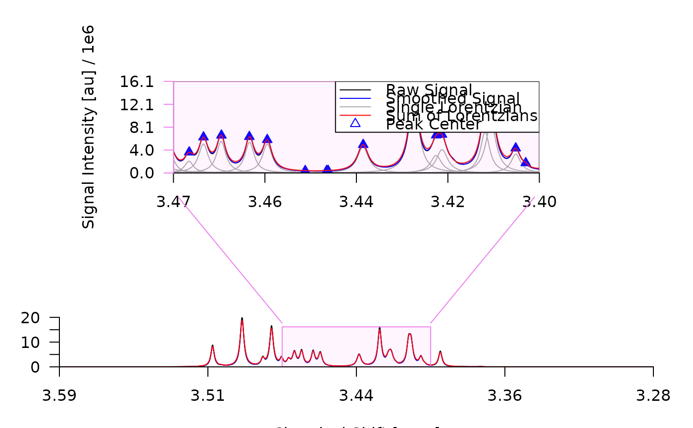
## 2.4. Change color of focus rectangle and margins of sub figure 1
## 2.5. Hide xlab and show second derivative
## 2.6. Change the figure region for sub figure 1
plot_spectrum(spec, sub1 = FALSE)
 plot_spectrum(decon, foc_rgn = c(3.49, 3.45), con_lines = FALSE)
 plot_spectrum(decon, sub2 = TRUE, foc_frac = c(0.40, 0.30))
 plot_spectrum(decon,
sub1 = list(mar = c(3, 6, 3, 6), lt_axis = list(col = "violet")),
foc_rect = list(border = "violet", col = transp("violet")),
con_lines = list(col = "violet")
)
 plot_spectrum(decon,
sub2 = TRUE,
sub3 = list(bt_text = list(text = "")),
frame = TRUE,
con_lines = FALSE
)
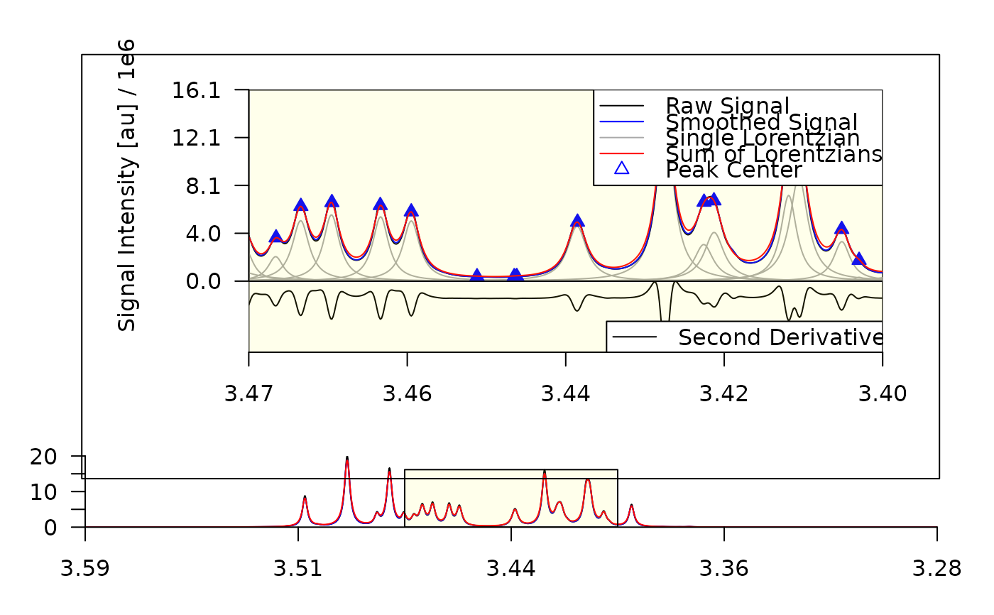 plot_spectrum(decon, sub1 = list(fig_rgn_npc = c(0,1,.3,1), mar = c(0,5,0,0)))
